high-pass filter

A high-pass filter (HPF) is an electronic filter that passes signals with a frequency higher than a certain cutoff frequency and attenuates signals with frequencies lower than the cutoff frequency. The amount of attenuation for each frequency depends on the filter design. A high-pass filter is usually modeled as a linear time-invariant system. It is sometimes called a low-cut filter or bass-cut filter. High-pass filters have many uses, such as blocking DC from circuitry sensitive to non-zero average voltages or radio frequency devices. They can also be used in conjunction with a low-pass filter to produce a bandpass filter.

First-order continuous-time implementation

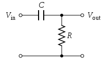
Figure 1: A passive, analog, first-order high-pass filter, realized by an RC circuit

The simple first-order electronic high-pass filter shown in Figure 1 is implemented by placing an input voltage across the series combination of a capacitor and a resistor and using the voltage across the resistor as an output. The product of the resistance and capacitance (R×C) is the time constant (τ); it is inversely proportional to the cutoff frequency f_c, that is,

${\displaystyle f_{c}={\frac {1}{2\pi \tau }}={\frac {1}{2\pi RC}},\,}$

where f_c is in hertz, τ is in seconds, R is in ohms, and C is in farads.

Figure 2: An active high-pass filter

Figure 2 shows an active electronic implementation of a first-order high-pass filter using an operational amplifier. In this case, the filter has a passband gain of -R₂/R₁ and has a cutoff frequency of

${\displaystyle f_{c}={\frac {1}{2\pi \tau }}={\frac {1}{2\pi R_{1}C}},\,}$

Because this filter is active, it may have non-unity passband gain. That is, high-frequency signals are inverted and amplified by R₂/R₁.

Discrete-time realization

For another method of conversion from continuous- to discrete-time, see Bilinear transform.

Discrete-time high-pass filters can also be designed. Discrete-time filter design is beyond the scope of this article; however, a simple example comes from the conversion of the continuous-time high-pass filter above to a discrete-time realization. That is, the continuous-time behavior can be discretized.
From the circuit in Figure 1 above, according to Kirchhoff's Laws and the definition of capacitance:

${\displaystyle {\begin{cases}V_{\text{out}}(t)=I(t)\,R&{\text{(V)}}\\Q_{c}(t)=C\,\left(V_{\text{in}}(t)-V_{\text{out}}(t)\right)&{\text{(Q)}}\\I(t)={\frac {\operatorname {d} Q_{c}}{\operatorname {d} t}}&{\text{(I)}}\end{cases}}}$

where ${\displaystyle Q_{c}(t)}$ is the charge stored in the capacitor at time ${\displaystyle t}$. Substituting Equation (Q) into Equation (I) and then Equation (I) into Equation (V) gives:

${\displaystyle V_{\text{out}}(t)=\overbrace {C\,\left({\frac {\operatorname {d} V_{\text{in}}}{\operatorname {d} t}}-{\frac {\operatorname {d} V_{\text{out}}}{\operatorname {d} t}}\right)} ^{I(t)}\,R=RC\,\left({\frac {\operatorname {d} V_{\text{in}}}{\operatorname {d} t}}-{\frac {\operatorname {d} V_{\text{out}}}{\operatorname {d} t}}\right)}$

This equation can be discretized. For simplicity, assume that samples of the input and output are taken at evenly spaced points in time separated by ${\displaystyle \Delta _{T}}$ time. Let the samples of ${\displaystyle V_{\text{in}}}$ be represented by the sequence ${\displaystyle (x_{1},x_{2},\ldots ,x_{n})}$, and let ${\displaystyle V_{\text{out}}}$ be represented by the sequence ${\displaystyle (y_{1},y_{2},\ldots ,y_{n})}$ which correspond to the same points in time. Making these substitutions:

${\displaystyle y_{i}=RC\,\left({\frac {x_{i}-x_{i-1}}{\Delta _{T}}}-{\frac {y_{i}-y_{i-1}}{\Delta _{T}}}\right)}$

And rearranging terms gives the recurrence relation

${\displaystyle y_{i}=\overbrace {{\frac {RC}{RC+\Delta _{T}}}y_{i-1}} ^{\text{Decaying contribution from prior inputs}}+\overbrace {{\frac {RC}{RC+\Delta _{T}}}\left(x_{i}-x_{i-1}\right)} ^{\text{Contribution from change in input}}}$

That is, this discrete-time implementation of a simple continuous-time RC high-pass filter is

${\displaystyle y_{i}=\alpha y_{i-1}+\alpha (x_{i}-x_{i-1})\qquad {\text{where}}\qquad \alpha \triangleq {\frac {RC}{RC+\Delta _{T}}}}$

By definition, ${\displaystyle 0\leq \alpha \leq 1}$. The expression for parameter ${\displaystyle \alpha }$ yields the equivalent time constant ${\displaystyle RC}$ in terms of the sampling period ${\displaystyle \Delta _{T}}$ and ${\displaystyle \alpha }$:

${\displaystyle RC=\Delta _{T}\left({\frac {\alpha }{1-\alpha }}\right)}$.

Recalling that

${\displaystyle f_{c}={\frac {1}{2\pi RC}}}$ so ${\displaystyle RC={\frac {1}{2\pi f_{c}}}}$

then ${\displaystyle \alpha }$ and ${\displaystyle f_{c}}$ are related by:

${\displaystyle \alpha ={\frac {1}{2\pi \Delta _{T}f_{c}+1}}}$

and

${\displaystyle f_{c}={\frac {1-\alpha }{2\pi \alpha \Delta _{T}}}}$.

If ${\displaystyle \alpha =0.5}$, then the ${\displaystyle RC}$ time constant equal to the sampling period. If ${\displaystyle \alpha \ll 0.5}$, then ${\displaystyle RC}$ is significantly smaller than the sampling interval, and ${\displaystyle RC\approx \alpha \Delta _{T}}$.

Algorithmic implementation

The filter recurrence relation provides a way to determine the output samples in terms of the input samples and the preceding output. The following pseudocode algorithm will simulate the effect of a high-pass filter on a series of digital samples: